Ch.2 – Spreadsheet

Download PDF File : Click here

Download Malayalam PDF File : Click here

SPREADSHEET

Spreadsheet   application   is   a   computer   program   that   allows   us   to   record,calculate and compare numerical or financial data. A spreadsheet is a configuration of   rows   and   columns.   Rows   are   horizontal   vectors   while   columns   are   vertical vectors.. LibreOffice Calc, MS Office Excel, Open Office Spreadsheet, etc. are examples of Spreadsheet software.

Workbook

A file in spreadsheet is known as a “Workbook”. A workbook is a collection of a number of “Worksheets”.

Worksheet

A page in a workbook is called Worksheet. It  is a collection of cells where you can keep and manipulate the  data. we  can add  as  many worksheets  as the memory capacity of our computer.

LibreOffice Calc

LibreOffice Calc  is a spreadsheet application that you can use to calculate, analyse, and manage data. It includes in  LibreOffice Package,   which is   Free and Open Source software under the General Public Licence (GPL)

Features of LibreOffice Calc

1. Easy calculation:-

It can perform complex calculations with ease.

2. What -if Calculations:-

Calc lets users to predict what will happen if certain conditions change.

3. Serve as a Database:-

Huge volume of data can be organised , stored and filtered without much efforts.

4. Arranging data asper user requirement:-

The stored data can be organised or reorganised according to the needs of the users.

5. Can provide dynamic Charts:-

Different inbuilt charts and graphs are available for presenting the data in appealing manner.

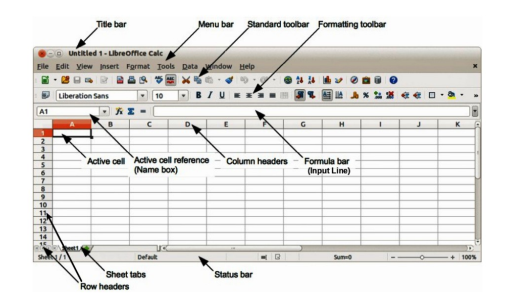
Components of LibreOffice Calc

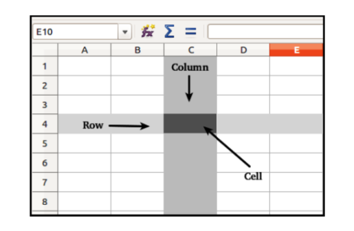
Row

A row is the range of cells that go horizontally in a worksheet.  Rows are identified by numbers like 1, 2,3 and so on.There are 10,48,576 rows are in Calc.

Column

A column is the range of cells that go vertically in a worksheet.  Columns are identified by letters like A, B, C  and so on. When it reaches Z, the next columns are identified as AA, AB, AC and so on.In Calc there are 1024 columns  named  as A to AMJ in a single worksheet.

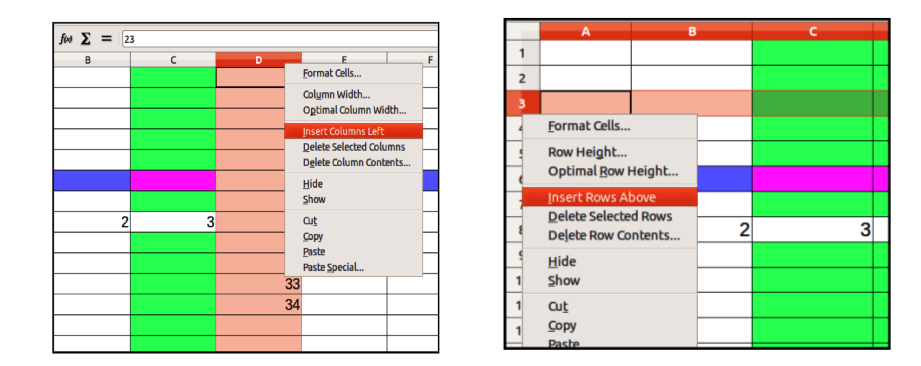
Inserting Rows and Columns

We can add or delete Rows and columns in a Spreadsheet. To add a column,click at the column header (right click on the mouse), there we get an option to add column. Likewise we can add row.

                  Insert column                     Insert row

Cell

Each rectangular box in a worksheet is referred  to as a cell. In other  words a cell is the intersection point of a column  and   row. Data entered  into Calc  is always stored in a cell. To keep track of where data is stored, each cell has a cell reference consisting of the column letter and row number of where the cell is located. Ex: A10

Range

Range is a group or block of cells. Ranges are identified by the cell references of the cell in the upper left and lower right corners of the range. These two references  are separated  by a colon ( : )

For example, the range D1:E10 includes a block of 20 cells starting from D1 and ending to  E10.

Naming Ranges

This means giving a name to a specific range.For example , scores obtained by students in Accounting is given in in the range C2:C10 , you can name this range as “Marks” also this name can be used in formulas and functions instead of quoting cell range as C2:C10.

For video Click here or scan QR code

Types of worksheet Data 

1- Value

 Value is a number that you enter in a cell.Thus numerical data is called a value.It also include currency symbol,minus,plus signs,decimal points and comma.

2- Labels

The text data is called label.It includes alphabets and symbols.they are non-numeric data but may include digits also. Ex: Name, Date of Birth , Mark etc.

3- Formula

Formulas are self-defined instructions entered  in cell for performing calculations. Formula should begin with an ‘= ‘ sign.  Ex =A1+B1

Components of a Formula

A standard formula may have three components

1. Cell Reference
2. Mathematical operators
3. Functions

1 – Cell Reference

To identify the location  of a cell, a reference  is given to a cell. It is also referred to as Cell Address. A cell reference or cell address consists of the column letter and row number that intersect at the cell’s location.    Ex : A1,E11,X18

Relative Cell Reference

Normally, when a formula or function from one cell is copied to another,  the references  given in the formula or function automatically changes to suit the new locations.  This type of reference is called Relative Reference.

Absolute Cell Reference

Unlike relative references,  absolute  references  do not change when copied to another  location. You can use  an  absolute  reference  to  keep  a row and/or column constant.  An  absolute  reference  is designated in a formula by the addition of a dollar sign ($). Ex: $A$1

Mixed Cell Reference

It  is a combination of relative and absolute Cell references that holds either row or column constant when the formula or function is copied to another location.This is known as mixed reference.  Ex:$A1  ,  B$10

 For video Click here or scan QR code

Basic and Derived Values

 If we directly enter  a value or piece of data in a cell, it is called Basic Value. If the data in a cell is generated  by an arithmetical expression or as the result of a function or formula, it is called derived value.

2 – Mathematical Operators

1. Arithmetic
2. Comparison
3. Reference

Operation Performed	Operator Symbol
Arithmetic OperatorsAdditionSubtractionMultiplicationDivisionPercentExponential	+–*/%^
Comparison OperatorsEqual toGreater thanLess thanGreater than or equal toLess than or equal toNot equal to	=><>=<=<>
Reference Operators Range OperatorsUnion operators	:,

3 – Functions

A function is a predefined formula which can be written directly into a cell, to display an outcome. which starts with ‘ Equal to sign’(=)Ex: SUM,MAX, MIN etc

Important Predefined functions in calc

1. Date and time function
2. Statistical Functions
3. Logical Functions
4. Mathematical Functions
5. Text  Functions
6. Spreadsheet Functions
7. Financial functions

1- Date and Time functions

This  function is used to perform operations on date and time values..The important date and time functions are TODAY(),NOW(),  DAY()  ,MONTH(), YEAR(), DATEVALUE()

TODAY()

This function shows current computer system date in the cell.The current date is automatically returned when we open the document on a future date. its  syntax is =TOADAY ()

Eg: in cell A1 if we enter =TODAY() it gives the result of today’s date ie, current system date. 26/09/2019

NOW()

NOW function displays the current system date and time. its Syntax is =NOW(). in cell A1 if we enter =NOW() it gives the result of today’s date and time, current system date and time. 26/09/2019 10:45

YEAR()

YEAR function returns the ‘year’from the date or date value given in the brackets. its Syntax is =YEAR(“Date” or Cell reference)  It ranges from 1900 to 9999.For example in the above case Year(A1) results in 2019. Ie; the 2018^th year.

MONTH()

This function shows the serial number of the month ranging from 1 to 12.   its Syntax is =MONTH(“date” or Cell reference).For example in the above case Month(A1) returns 9, i.e. the 9^th month

DAY()

 it shows the day of the date.Its syntax is =DAY()  (“Date” or cell reference). For example if A1 = 26/09/2019, the Day(A1) will result in 26. Because it is the 26^rd day of the month.

DATE VALUE

 This function converts the given date to the corresponding value.LibreOffice calc considers 30/12/1899 as the base date with date value zero(0) .The syntax is =DATEVALUE(“ date”)

 For example we enter in cell A1 =DATEVALUE(“26/09/2019”) It gives the result of 43734. There are 43734 days from 30/12/1899 to 26/09/2016.

DATE

 This function returns a date, when the year ,month and day parameters are given as integer seperated by commas.

Syntax : DATE(Year,Month,Day)

Ex : DATE(2019,09,26) it is displayed as 26/09/19

For video Click here or scan QR code

2- Statistical Functions

Statistical function operates on a set of data and gives summarised results.

COUNT()

 The  COUNT  function  will  count  cells  that  contain  numbers  or  count  the  numbers given  in  the arguments separated  by commas.Only numbers,dates and time are counted here.

 The syntax is       =COUNT(A1:B5)  or

                           =COUNT(Value1; Value2; … Value30)

 Value1; Value2, … are 1 to 30 values or ranges representing the values to be counted.

COUNTA()

The COUNTA function counts the  number  of cells that  contain any type of data.  In other  words it counts the number of cells that are not empty in a range. The cells that contain a formula, but the result as empty (” “) is also counted here.

Syntax is      =COUNT(A1:B5) 

                  =COUNTA(Value1; Value2; … Value30)

Value1; Value2, … are 1 to 30 arguments representing the values to be counted.

COUNTBLANK()

 COUNTBLANK  function  counts  the  number  of empty cells in a range.  It  is an opposite function of COUNTA. A cell that contains formula is not treated  as empty, even if its result is empty.

 Syntax is =COUNTBLANK(Range)

  Returns the number of empty cells in the range.

COUNTIF()

This function counts the number of cells within a range that meet the given criteria or condition. here the blank cells and text values are ignored.

 Syntax is =COUNTIF(range,criteria)

AVERAGE

Average is calculated by adding a group of numbers and then divided by the count of those numbers 

Content in the Cell B1	Content in the Cell C1	Content in the Cell D1	Function in Cell E1	Result in Cell E1
20	30	40	=AVERAGE(B1:D1)	30

MIN()

It finds the smallest number in a set of values

Content in the Cell B1	Content in the Cell C1	Content in the Cell D1	Function in Cell E1	Result in Cell E1
20	30	40	=MIN(B1:D1)	20

MAX() 

It finds the largest number in a set of values.

Content in the Cell B1	Content in the Cell C1	Content in the Cell D1	Function in Cell E1	Result in Cell E1
20	30	40	=MAX(B1:D1)	40

 For video Click here or scan QR code

3 – Logical Function

Logical functions are used to compare two values or statements.The commonly used logical functions are IF,AND and OR

IF()

The IF function is one of the most popular and useful functions. IF function  test a condition and to 

return one value if the condition is true, and another value if the condition is false.

Syntax

IF(Test, ThenValue, OtherwiseValue)

Test is logical test.

ThenValue (optional) is the value that is returned if the logical test is TRUE.

OtherwiseValue (optional) is the value that is returned if the logical test is FALSE.

Marks	Function	Result
50	=IF(A2=>30,”PASSED”.”FAILED”)	PASSED
25	=IF(A3=>30,”PASSED”.”FAILED”)	FAILED

NESTED IF

An “IF” within another ”IF” function statement, it is known as “NESTED IF”. If first condition is false it is checked next and if the second condition is false it is check next and so on.

Marks	Function	Result
90	=IF(A2>=90,”A+”,IF(A2>=80,”A”,IF(A2>=70,”B+”,IF(A2>=60,”B”,IF(A2>=50,”C+”,IF(A2>=40,”C”,IF(A2>=30,”D+”,”D”)))))))	A+
25	=IF(A2>=90,”A+”,IF(A2>=80,”A”,IF(A2>=70,”B+”,IF(A2>=60,”B”,IF(A2>=50,”C+”,IF(A2>=40,”C”,IF(A2>=30,”D+”,”D”)))))))	D

AND

This function checks more than one condition at the same time and returns TRUE if all the conditions are satisfied. Otherwise it Returns FALSE.

Syntax

AND(LogicalValue1; LogicalValue2 …LogicalValue30)

LogicalValue1; LogicalValue2 …LogicalValue30 are conditions to be checked. All conditions can be either TRUE or FALSE.

OR

Returns TRUE if any argument is TRUE; returns FALSE if all arguments are FALSE.

syntax: =OR(LogicalValue1; LogicalValue2 …LogicalValue30)

LogicalValue1; LogicalValue2 …LogicalValue30 are conditions to be checked. All conditions can be either TRUE or FALSE. 

For video Click here

4 – Mathematical Functions

These functions are used for arithmetical calculations mostly used in business. it includes SUM,ROUND etc.

SUM()

It is used to add all the numbers in a range of cells. 

=SUM(A1:A10) it adds the numeric values from cell A1 to Cell A10.

=SUM(10,15) It add the values 10 and 15,ie 25

=SUM(Range1,Range2…….

SUMIF()

SUMIF Function ADD the cells specified by a given criteria

 Syntax is =SUMIF(range,”criteria”,sum_range)

For video Click here

Range is the range to which the criteria are to be applied.

Criteria is the cell in which the search criterion is shown,  If the criteria is written into the   formula, it has to be surrounded by double quotes.

SumRange is the range from which values are summed. 

ROUND()

It rounds a number to a specified number of digits asper normal rounding rules,i.e.; round down if the decimal portion is < 5, and round up if the decimal portion is ≥5

Syntax is =ROUND(Number,Count)

Number – The number that you want to round

Count   – The number of digits to which you want to round the number.

Ex:

=ROUND(2.348,2) returns 2.35

=ROUND(-32.4834,3) returns -32.483. Change the cell format to see all decimals.

=ROUND(2.348,0) returns 2.

=ROUND(2.5) returns 3.

=ROUND(987.65,-2) returns 1000.

=ROUND(4.15,1) Rounds 4.15 to one decimal place  4.2.

ROUNDUP()

This function is similar to ROUND function.This function rounds a number up away from zero. If the number  in rounding position  is more than zero, it is rounded  to the next.

Ex:

=ROUNDUP(1.1111,2) returns 1.12.

=ROUNDUP(1.2345,1) returns 1.3.

=ROUNDUP(45.67,0) returns 46.

=ROUNDUP(-45.67) returns -46.

=ROUNDUP(987.65,-2) returns 1000.

ROUNDDOWN()

Round a number down  towards zero.This function always round a number to downward, without considering the value next to the rounding digit. Eg. = Rounddown(125.675, 1) 

results in 125.6

For video  Click here or scan QR Code

Ex:

=ROUNDDOWN(1.234,2) returns 1.23.                                                             

=ROUNDDOWN(45.67,0) returns 45.

=ROUNDDOWN(-45.67) returns -45.

=ROUNDDOWN(987.65;-2) returns 900.

5- Text  functions

This functions are used for creating or modifying the data entered in cells to a required text format.

TEXT()

TEXT function Converts a number into text according to a user  given format.It helps to display numbers in a more readable format.

Syntax =TEXT(Number; Format)

Number is the numerical value to be converted.

Format is the text which defines the format. Use decimal and thousands separators according to the language set in the cell format.

For video Click here

Ex:

=TEXT(12.34567;”###.##”) returns the text 12.35

=TEXT(12.34567;”000.00″) returns the text 012.35

CONCATENATE()

Combines several text strings into one string.

Syntax

                  =CONCATENATE(“Text1”, …, “Text30”)

Text 1; Text 2; … represent up to 30 text passages which are to be combined into one string.

Example

=CONCATENATE(“Good “,”Morning “,”Mrs. “,”Rani”) returns: Good Morning Mrs. Rani.

6 – Spreadsheet  Functions

LOOKUP

LOOKUP function is used for searching certain values from a particular table.

LOOKUP function has two syntax forms,they are:

1. Vector form and 2) Array form

LOOKUP(Vector form)

Syntax

LOOKUP(SearchCriterion,SearchVector,ResultVector)

SearchCriterion is the value to be searched for; entered either directly or as a reference.

SearchVector is the single-row or single-column area to be searched.

ResultVector is another single-row or single-column range from which the result of the function is taken

For video Click here

LOOKUP(Array form)

An array is a linked range of cells on a spreadsheet containing values.The smallest possible array is 1X2 or 2X1 array with two adjacent cells.

Syntax is =LOOKUP(lookup_value,array)

                  For video Click here or scan QR code              

VLOOKUP

This function checks if a specific value is contained in the first column of an array. The function then returns the value in the same row of the column named by Index

Syntax

   =VLOOKUP(SearchCriterion,Array,Index,SortOrder)

SearchCriterion  –  the value you are looking for in the first column of the array.

Array                  – Where you are looking     

Index                  –  is the number of the column in the array that contains the value to be returned. The first column has the number 1.

SortOrder     – Precise or approximate values will be returned.Give ‘0’ for precise value and ‘1’ stands for approximate value.

For video Click here or scan QR code

HLOOKUP

Searches for a value in the top row of table/array of values,and returns a value in the same column from the row,named as Index.

For video Click here or scan QR code

Syntax

HLOOKUP(SearchCriteria,Array,Index,Sorted)

SearchCriterion is the value searched for in the first column of the array.

Array is the reference, which is to comprise at least two columns.

Index is the number of the column in the array that contains the value to be returned. The first column has the number 1.

SortOrder Indicates whether to find an exact match.True or 1 gives closest match and False or 0 returns exact match.

ROWS

This function gives back the number of rows when this function is used on a range of cells.

Syntax : =ROWS(Array)

Ex : ROWS(C1:H4)  the result is 4

COLUMNS

This function returns the number of columns in an array or reference.

Syntax =COLUMNS(Array)

Ex : COLUMNS(C1:H4)  the result is 6

For video Click here or scan QR code

7 – Financial functions

This category contains the  finance functions of LibreOffice Calc.

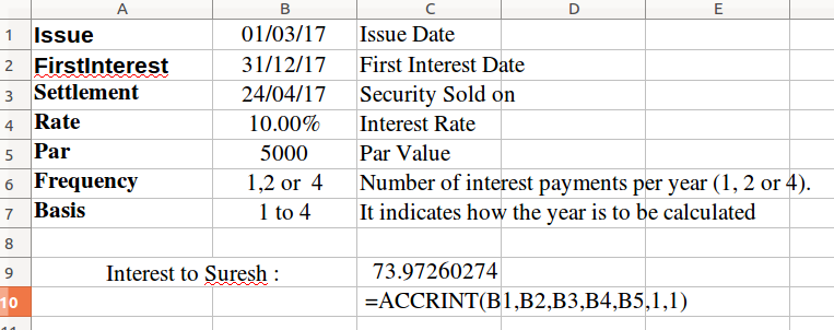
ACCRINT

Calculates the accrued interest of a security in the case of periodic interest.Accrued interest is interest due but not received/paid.Companies may pay interest on debentures or bonds periodically( quarterly,half yearly or yearly).If a holder sells his security before next interest due date,the buyer has to pay its market value and plus interest earned up to the settlement date. ACCRINT function helps to calculate  such interest easily.

Syntax

ACCRINT(Issue,FirstInterest,Settlement,Rate,Par,Frequency, Basis)

Issue is the issue date of the security.

FirstInterest is the first interest date of the security.

Settlement  – The settlement date of the security(ie. sold or purchased)

Rate is the annual  rate of interest (coupon interest rate)

    Par is the par value of the security.

   Frequency is the number of interest payments per year (1 for annual, 2for half yearly and 4 for  quarterly).

  Basis (Optional) It indicates how the year is to be calculated.If the basis not given it is automatically counted as zero.

Basis	Calculation
0	US method (NASD), 12 months of 30 days each
1	Exact number of days in months, exact number of days in year
2	Exact number of days in month, year has 360 days
3	Exact number of days in month, year has 365 days
4	European method, 12 months of 30 days each

Example:

On 1.Mar.2017, Mr.Suresh has invested Rs.5000 in a security having compound interest @10% annually. The next interest date of the security is 31-Dec-2017. But meanwhile on 24-April-2017 he sold  the security to Mr.Mahesh. On 31st Dec 2017, Mr.Mahesh will get interest for the 9 months. But Mr.Suresh was the holder of the security for 54 days and hence Mr.Mahesh has to pay interest receivable for these days to Suresh, along with the market value of the security. This interest is

                    = 5000 X 10100X 54365= 73.97260274  

RATE

Calculate the  interest rate per period of an annuity.

Syntax

=RATE(NPer,Pmt,PV,FV,Type,Guess)

Nper   – Total number of payment periods

PMT   – payment made each period.Given as minus figure.

Pv       – the total amount

Fv      – Future value or cash balance after the last payment

Type  – 1 for beginning and 0 for the end of the period.

Guess –  Is your guess for what the rate will be, by default it is 10%

Asha Menon taken a loan of 500,000 from CANARA Bank, agreed to pay 

11,500 per month over a period of 5 years, and the monthly payments are to be made at the end of each month. Compute the rate of interest using Rate Function.

CUMIPMT

Returns the cumulative interest paid on a loan between two dates.

Syntax

CUMIPMT(Rate, NPer, PV, S, E, Type)

Rate is the periodic interest rate.(if annual rate is given,find monthly rate)

NPer is the length of loan in months (if given in years to be converted in to months).

PV is the current value in the sequence of payments.

S is the first period.

E is the last period.

Type is the due date of the payment at the beginning(1) or end(0) of each period.

Example :

A loan of Rs 5,00,000 was taken on  01-01-2017.The annual Interest rate is 10%, The loan is repayable in monthly instalment over 4 years.

To calculate the interest payable in first 8 months:-

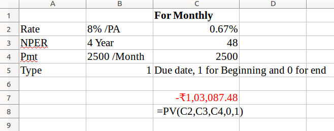
PV

This function is used to calculate the amount of money needed to be invested at a fixed rate today, to receive a specific amount, over a specified number of periods

Syntax

=PV(Rate,NPER,Pmt,FV,Type)

Rate defines the interest rate per period(if annual rate is given,find monthly rate).

NPER is the total number of periods (payment period).

Pmt is the regular payment made per period(Pmt should be given as negative as it is payment)

FV (optional) defines the future value ,or a cash balance to attain after the last payment is made.

Type (optional) denotes due date for payments(1 for beginning and 0 for the end of the month)

Example

Anil opened a Recurring Deposit Scheme paying Rs.2500 per month for a period of 4 years with an interest rate of 8% per annum, and the payments are made at the beginning of

PMT

This function calculates the payment for a loan based on constant payments and a constant interest rate.

Syntax is :

=PMT(Rate,Nper,PV,FV,Type)

Rate is the periodic interest rate (if annual rate is given,find monthly rate)

Nper is the number of periods over which the loan or investment is to be paid.

PV is the present value of loan or investment.

FV (optional) is the desired value (future value) to be reached at the end of the periodic payments

Type (optional) is the due date for the periodic payments. 1 for beginning and 0 for end of the period.

Example

Calculate the Monthly payment for a Loan of 25,000 taken  by Raju from SBI with an interest rate @ 8% for a period of 3 years.

FV

This function calculates the future value of an investment based on periodic,constant payments and a constant interest rate.

Syntax

                =FV(Rate,Nper,Pmt,PV,Type)

Rate is the periodic interest rate.

NPer is the total number of periods (payment period).

Pmt is the annuity paid regularly per period.

PV (optional) is the (present) cash value of an investment.

Type (optional) defines whether the payment is due at the beginning or the end of a period.

Example:

 Anil  has made a periodical payment of ₹750 with an interest rate at 4% for a period of 2 years. What is the Value at the end(Future Value).

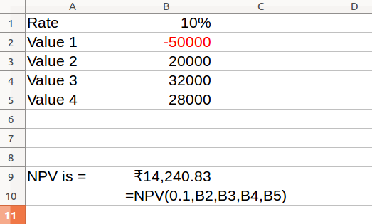
NPV

Returns the present value of an investment based on a series of periodic cash

flows and a discount rate. For example,if interest rate is 10%,the value of Rs.1000 received after one year is only Rs.909.That means if we invest Rs.909 today,we will get Rs.909+10% interest(Rs.999.9) after one year.

Syntax

          =NPV(Rate,Value1,Value2,…)

Rate is the discount rate for a period.

Value1;… are up to 30 values, which represent deposits or withdrawals.

Example:

A company invest Rs.50000 in a project at the end of this year it brings inflow of Rs.20000,32000,and 28000 respectively at the end of next three years. Here Net Present value is

Data Entry,Text Management and Cell Formatting

Data Entry

Entering Data in calc means Data entry. 

a – Direct Data entry

We can enter the data directly using keyboard.

b – Data fill options

In Calc, can fill Data automatically in cells with the Auto Fill command or series command.

(i) AutoFill

Libreoffice calc provides an option for entering data automatically with a series of numbers ,text and number combination ,dates,time periods based on a defined pattern.

For video Click here

(ii) Defined Series

We can also fill the active  ell with the content of an adjacent cell through the ‘Fill series window’.This Fill option is available in the ‘Edit’ menu

Enter in Cell A1 25 and select the range A1:A10, go to Edit -> Fill -> Series -> OK

(iii)Fill Handle

The ‘Fill’ command can be used to fill data into worksheet cells. (A Fill handle is the small black square in the lower­ right corner of the selection.When we point to the fill handle, the pointer changes to + symbol.and drag the fill handle across the cells that we want to fill.

c – Import/Copy Data from other sources

If you have data in an alternative source, you may be able to import it into Calc, instead of having to re-enter all the information again.

Click on ‘Sheet from File’ option from Insert menu. Select the text file or csv file with the help of dialogue box appears and press OK button, select the separator option then press OK.

For video Click here

Data Validation

Data validation is a feature to define restrictions on type of data entered into a cell. We can configure data validation rules for cells data that will not allow users to enter invalid data, There may be warning messages when users tries to type wrong data in the cell.

For video Click here

Data Form

We can also enter data into cells using ‘Data Input Form.It helps in data validation by reducing the chances of errors in data entry.Using a Data Form,we can make data entry more easy and accurate.

For video Click here

Data Formatting

Formatting means the arrangement of data for computer input or output,in terms of number and size of fields in a record. Formatting of spreadsheets makes easier to read and understand the important information.The worksheet data formatting may be in the following form.

1. Number Formatting

Numbers are formatted to change their appearance. Number formatting includes adding percent(%),comma,decimal places and currency sign,date,time scientific values etc to a spreadsheet.

For video Click here

2. Text Formatting

Text formatting is mostly required for presentation of final output.it can be used to display the text in different fonts,align the cells ,change font color, merge cells etc.

3. Conditional Formatting

The conditional formatting changes the appearance of a cell renage based on condition or criteria.If the specified condition is true,the cell range is formatted automatically. 

For video Click here or scan QR code

4. Table Formatting

This option formats a range of cells and converts it into a table by choosing a predefined table style.

For video Click here

Cell Formatting 

 Cell formatting means modification of cell or range of cells as desired by user.

Merging a range of Cells

Merged cells are a single cell that is created by combining two or more selected cells. The cell reference for a merged cell is the upper ­left cell in the original selected range.

For video Click here

Out put reports

Report is a document that conveys specific information to others.So it should be attractive ,legible and systematically presented.

Page Setup

We can customise our output Report by editing the page setup option.It can be accessed by

 Format (in the file menu)→Page

opens the Page Style window in the page tab.

Print Out

We can print entire or partial worksheets and workbooks, one at a time, or several at once.

Defining the Print Area

By default, LibreOffice Calc prints all data on the current worksheet but for specific and formatted print we have to define print area from the print Lay out from ‘File’ menu.

For video Click here

Print non-contiguous ranges

You can also print non-contiguous cells(cells which do not touch other) in a single sheet.

Select two or more ranges to be printed and click b Print.

For video Click here

One Variable Data Table

A One Variable data table is simply a table that shows multiple results, based on different source data.One variable Data Table is most suited in situations when you want to see how the final result changes when you change one of the input variables.

For video Click here

Two Variable Data table

Two Variable Data Table works similar to the One Variable Data Table.However, which specify two decision variables and a variety of inputs and only a single result.

For video Click here

Pivot Table

Pivot table is a tool for combining ,comparing and analysing large amounts of data easily. It is a table that summarizes source data in another table ,displays the details of areas of interest and create reports. A Pivot table allows you to create an interactive view to your data set.
Data can be arranged, rearranged or summarized according to different points of view.

Data → Pivot table→Create

For video Click here

Common Errors in Calc

Message	Error Code	Explanation
###		The cell is not wide enough to display the contents
#DIV/0!	532	If the denominator is 0
#NAME?	525	Excel doesn’t recognize the text in the formula.
#REF	524	Cell reference is invalid
#VALUE	519	The formula contains an inappropriate type of argument.
#NUM!	503	The formula contains an invalid number
#NULL		Invalid intersection
#NA		The formula cant display a value.

navas@comlive.in

www.facebook.com/comlive.in

www.youtube.com/c/comlive